This one is heavily grounded on what I suppose I master: simulation versus measurements, and most of all, free-field. Arrays of transducers — on lines, on screens, any way — are hyper-sensitive to their locations, phase, cancellation spots across frequency variations. But the thing was: I found a way to train a machine-learning module. The idea is simple, and you will have fun understanding it.
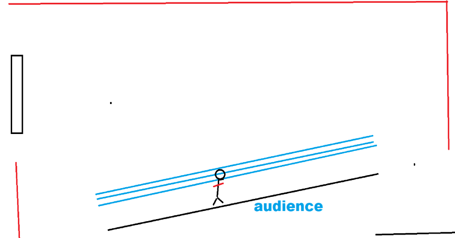
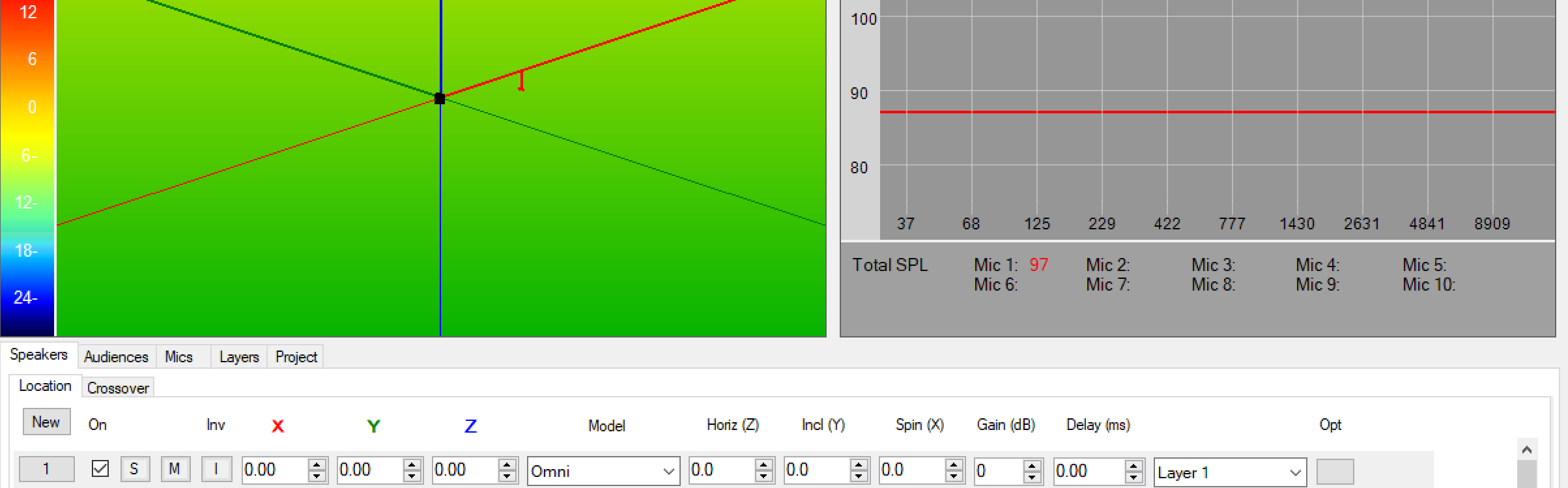
This image is important. The blue lines mark where we want sound. The red mark where we don't want sound, or crazy lobes. Everything downstream serves this map.
Why 2D is not a detour.
About the 2D view — we will not necessarily sell 2D columns like the Germans Fohhn or RH. But the theoretical analysis can prove very important because when we go from a line of sources (a column) to a screen of them (the Digital Horn), it becomes a matter of adding one more dimension to fairly simple equations. Analysis in 2D is always doable in 3D, and in 2D we save computing power by a lot — which lets research techniques be shown as they are below.
Algorithms are machines that transform data into transfer functions — delivered as FIR filters.— Digital Horn V2, the definition
On the image we have an 8-source line array, straight — what is any column by several players in the industry. The important thing is the syntax, or the way to call these algorithms, which we have learned: Algorithms are machines to transform data into delay/gain tables (Digital Horn V1). Or better — our algorithms create transfer functions to each transducer, delivered as generated FIR filters (Digital Horn V2), absolutely disconnected from V1.
Again, this is theoretical. It is good that we now have the 8 new transducers and we are preparing the Agata1 simple model to play with.
The biggest bet: active noise cancellation.
I would say my biggest bet for advanced toys (V2) is to actually create places with active noise cancellation, based on the method I have been developing and got to understand. On FIRs, there is a very easy way to send an echo of the signal — or two echoes, or as many echoes as the number of taps the FIR has to offer. But for our art — at least, starting — not more than four or five different duplications of the signal, each with their own very specific response. That last idea is the superposition: to add multiple echoes of the signal inside one simple FIR.
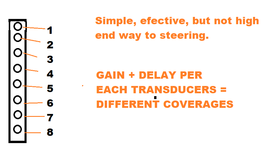
For our simple understanding and V1 approaches, this is the system. Most players in the industry work exactly like this.
Delays alone can already paint a coverage.
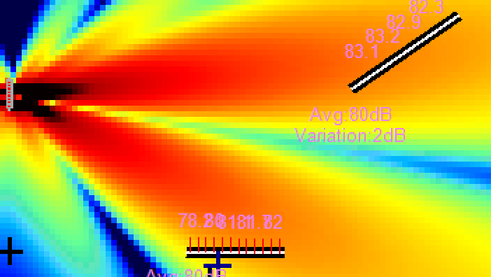
A variety of different coverages can already be created with delays and gains alone — let's see.
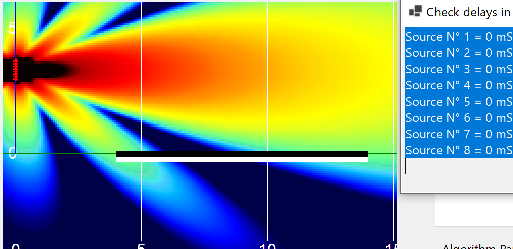
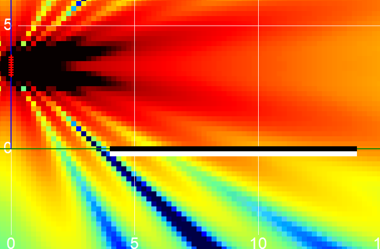
On each one we can see the delays applied. This is the natural response — zero delay on each source — at 1 kHz.
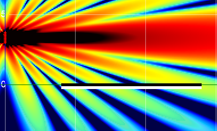
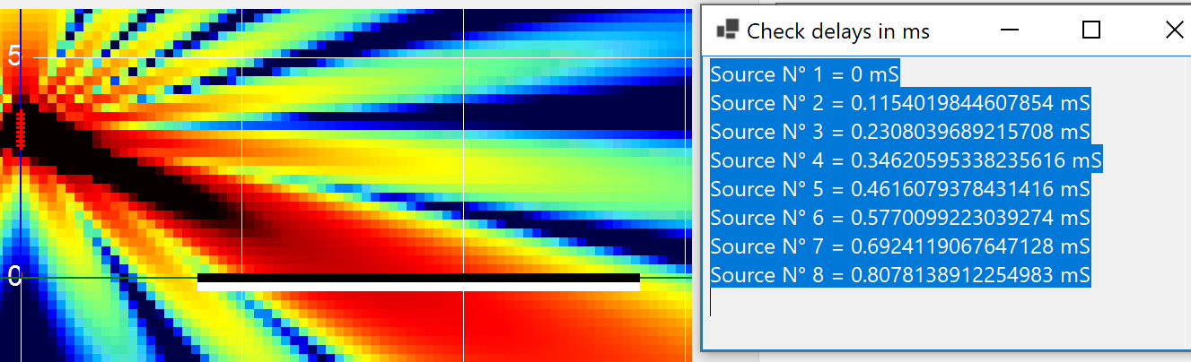
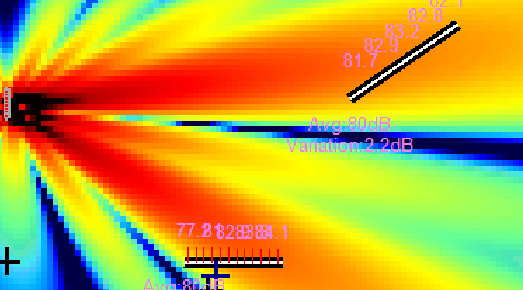
A nastier frequency in terms of directionality — the natural coverage at 2500 Hz.
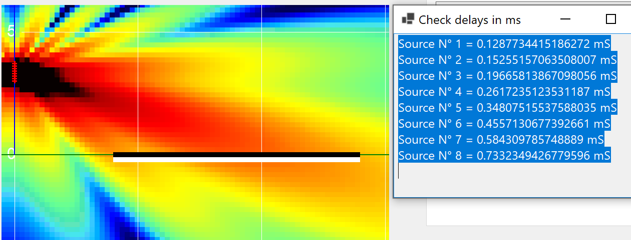
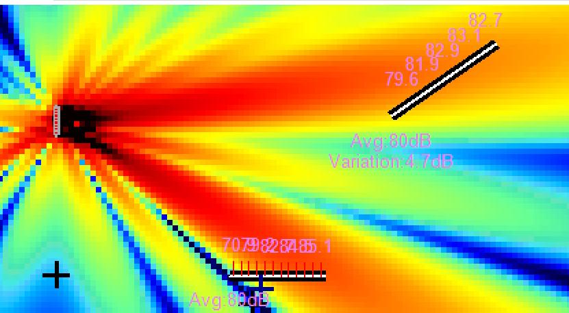
Same 2500 Hz — but with the delay values touched. The coverage opens.
Same location for the sources. Different coverage — only the numbers changed.
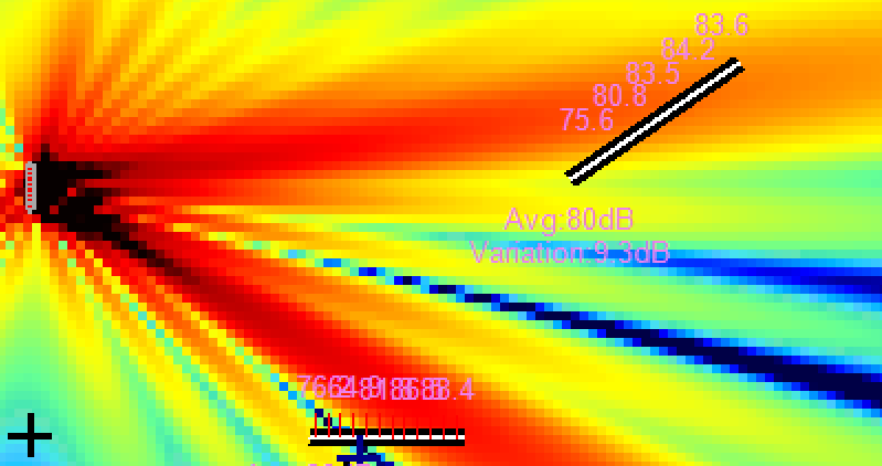
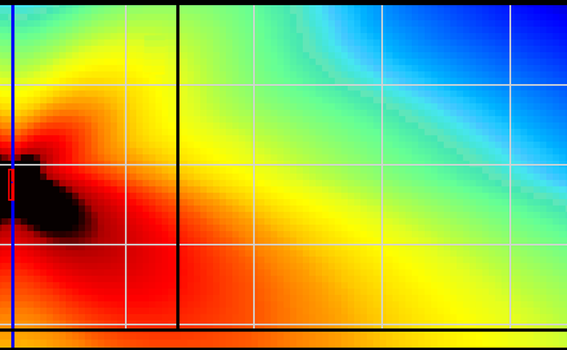
Directional plus open coverage. The area of interest has a "red" even SPL. This is when it starts to get interesting.
Multi-audience — the first real FIR trick.
FIR superposition techniques allow more advanced results such as typical multi-audience coverage.
1 kHz.
1250 Hz.
1600 Hz.
2000 Hz.
2500 Hz.
These are clearly an algorithm that, besides their crazy lobes, at any mentioned frequency covers the desired areas. But hey — these are two separated areas, and there is a clear separation of the beams. With more or less chaos, the differences are red to green to blue: that is a lot of decibels of difference, so the effect is created, and it is noticeable.
The thing here is that we are overthinking a simple delay/gain table. Here you need exactly two delay/gain tables — one for each direction of the sound beam. And in a while we will see the effect of more than two. To add magic: these tables are different for each frequency the FIR can manage. So, goodbye to the one-dimensional gain/delay-table algorithm.
A FIR is an impulse. An impulse is a transfer function. That is the only respectful algorithm.— the syntax of V2
Example — a simple FIR that produces an echo:
10000000000100000000000000000000
Number of taps: 32. This FIR is a superposition — it will send the signal being processed twice. Mental note: these multi-FIRs, when FFT'd, are not very fun to look at.
Example of a perfect impulse. The fun Omni model in Direct — good memories to understand sound summation beyond any polar-pattern or frequency-response effect. The response is flat.
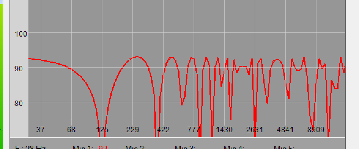
A 2-impulse superposition FIR — a 4 ms superposition, simple echo. Evidently, a comb-filter.
The thing is that each of these 8 (or N) comb-filters is different. But when combined —
— they sum on the desired directions, and the comb-filtered chaos of each source becomes order on the audience.
Much more can be done with this superposition technique — including, maybe, the holy grail: active muting of non-desired lobes (V2).
Active muting — the magic impulse.
We have data. We have separation between sources, and places where we want sound and places where we don't.
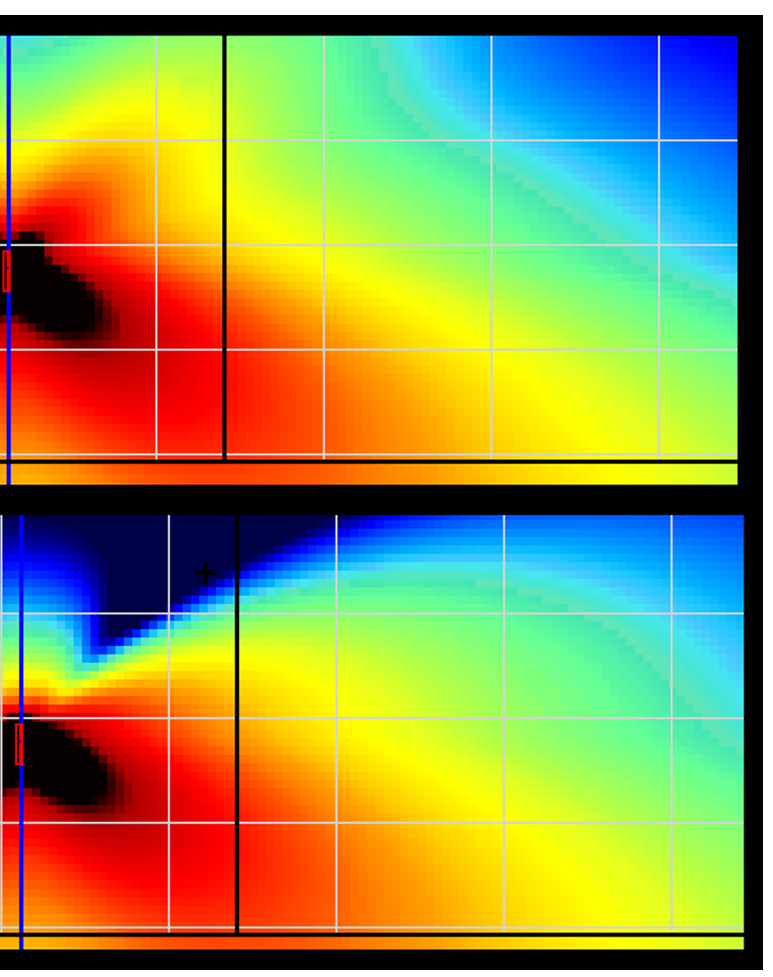
Upper image is the 1-impulse per source, natural and good response for some area. But there is an upper, crazy, powerful lobe that will take out intelligibility or simply the "promised" focused sound.
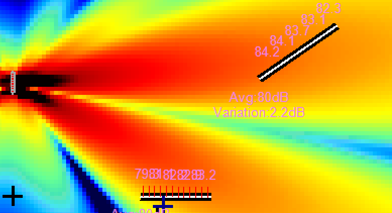
Now — the confidential: a tricky second impulse. And we got exactly this: transformation. Above, the original. Below, the magic.

This magic is just a second impulse — not made for covering a second area, but for muting the non-desired crazy roof lobe. For the effect to be effective, 1.5 dB were sacrificed. Efficient enough.
Next deliveries of the diaries I will show how to really get into this — which, still, I must say is a fairly complex task, because each frequency has different lobes for different coverage challenges.
The legend says — with a FIR, you have magnitude and phase independency across the frequencies you can control.