The governing picture. Sources on a line; audiences where we want sound; places we don't.
About the 2D view: we will not necessarily sell 2D columns like the Germans Fohhn or RH. But the theoretical analysis can prove very important, because when we go from a line of sources (2D) to a screen of them (3D, the Digital Horn), it is a matter of adding one dimension. Analysis in 2D is always doable in 3D, and in 2D we save a lot of computing power — which frees research for techniques shown below.
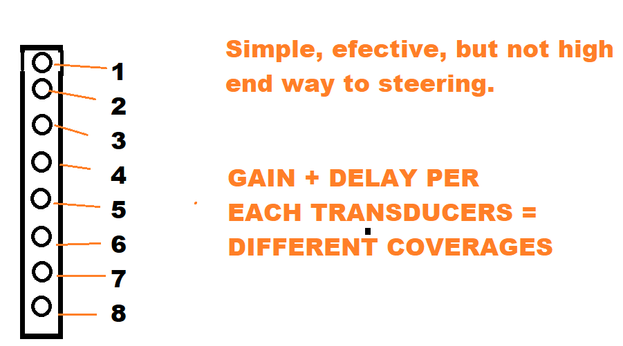
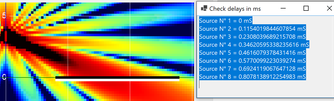
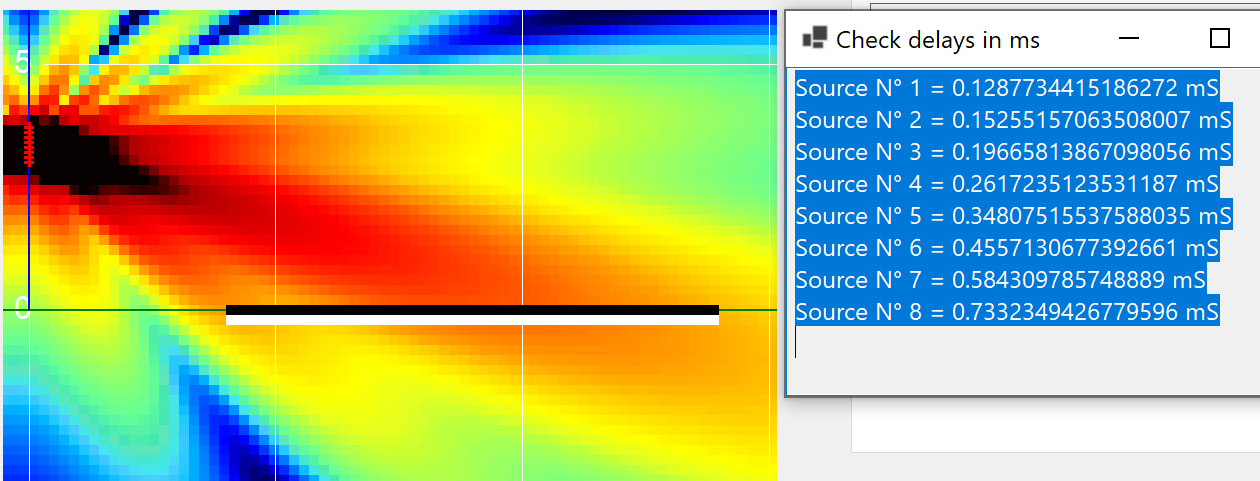
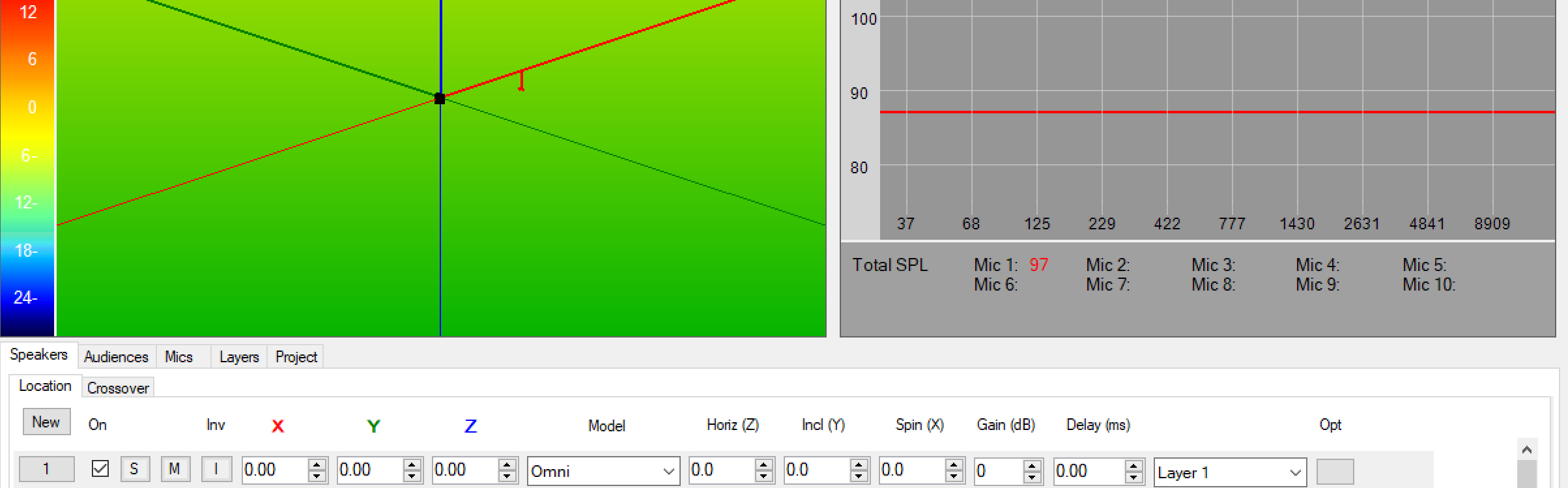
On the image we have an 8-source line array — what is any column by several players on the industry. The important thing is the syntax: Algorithms are machines to transform data into delay/gain tables (Digital Horn V1), or better — our algorithms create transfer functions to each transducer, delivered as generated FIR filters (Digital Horn V2), absolutely disconnected from V1.
My biggest bet for advanced toys (V2) is actually to create places with active noise cancellation, based on the method I have been developing. On FIRs, there is a very easy way to send an echo — or two, or as many as the number of taps the FIR has to offer. For our art, at least starting, not more than four or five different duplications of the signal, each with their own very specific response.
That last idea is superposition: to add multiple echoes of the signal inside a single FIR.
V1 — the approach most players in the industry use. One impulse (delay + gain) per source.
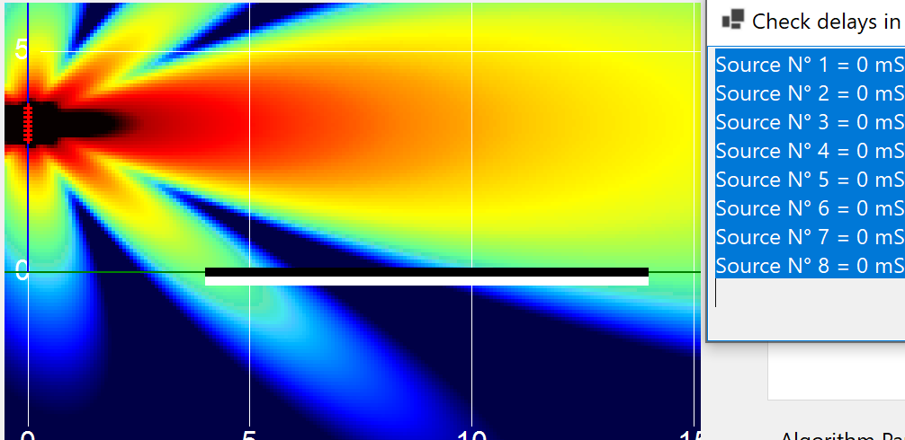
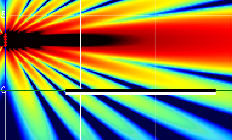
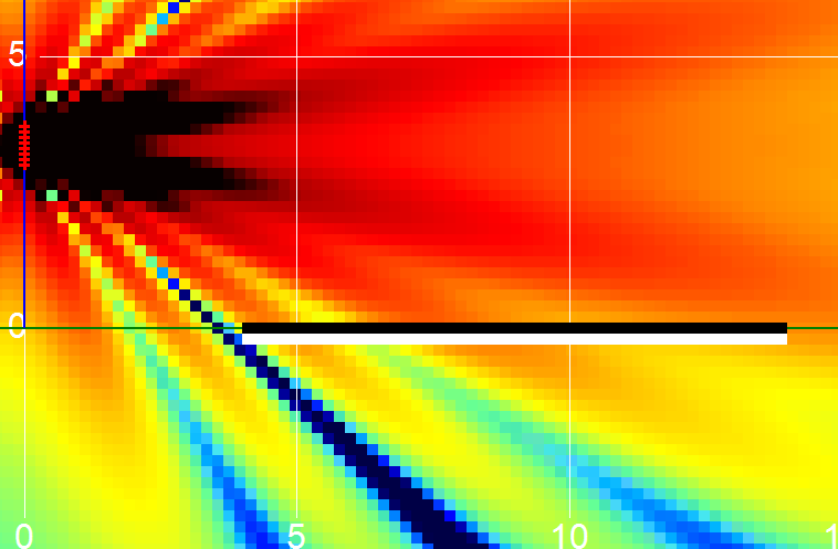
Delays paint the coverage.
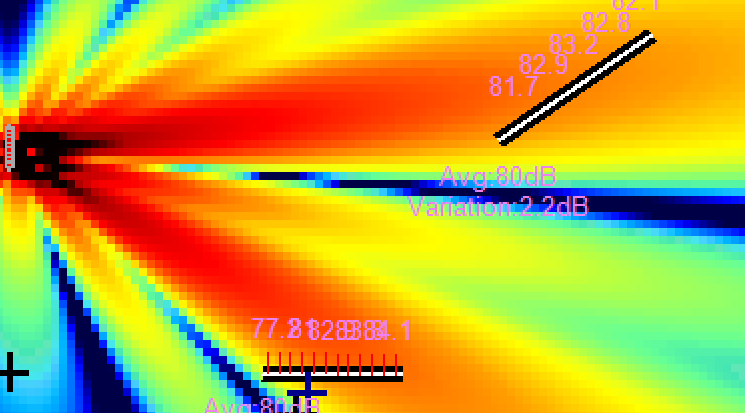
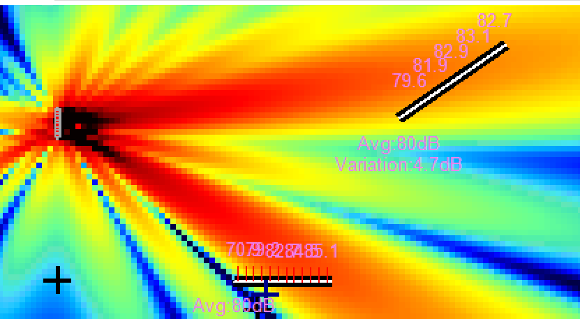
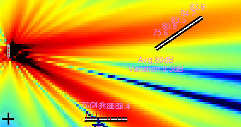
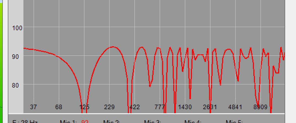
Natural response — zero delay each source, at 1 kHz.
Natural coverage at 2500 Hz — a nasty frequency in terms of directionality.
Same 2500 Hz — now with delay values touched. The coverage opens.
Same location for sources. Different coverage — only the numbers changed.
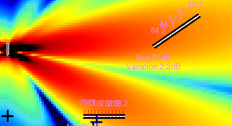
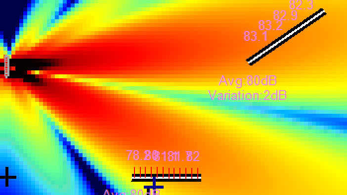
Directional plus open coverage. The area of interest now shows a "red" even SPL.
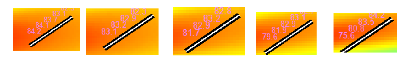
Multi-audience — across five frequencies.
FIR superposition allows more advanced results, such as typical multi-audience coverage.
1 kHz.
1250 Hz.
1600 Hz.
2000 Hz.
2500 Hz.
At any frequency, the algorithm covers the desired areas — and these are two separated areas with a clear separation of the beams. The lobes are crazy, but the differences are from red to green to blue: lots of decibels. The effect is created and it is noticeable.
The thing is we are overthinking a simple delay/gain table. Here you need exactly two delay/gain tables — one per beam direction. And in a while we will see more than two. To add magic, these tables differ for each frequency the FIR can manage. Goodbye to the one-dimensional gain/delay-table algorithm. The only respectful algorithm is the one which delivers a FIR.
Each comb-filter is different. When combined, they sum on the desired directions.— how the magic works
Example of a perfect impulse — the fun Omni model in Direct. The response is flat.
A 2-impulse superposition FIR — a 4 ms simple echo. Evidently, a comb-filter.
Each of these comb-filters is different — but when combined, they sum on the desired directions.
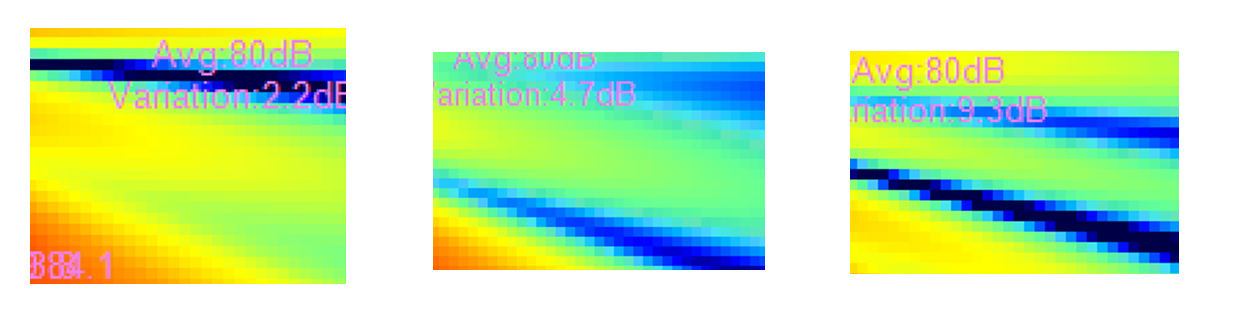
Balcony & main area.
To finish this informative one, look at the different required places, at very different frequencies. The balcony, I cut each SPL map at them.

The balcony slice, frequency by frequency.
And a place where we did not want the sound to concentrate — the part between the balcony and the main area.

Not the best, but there is a difference — and in advanced systems we will go for more of it. Those crazy lobes, tamed.
— The end.